Working with data in elite sport

class: bottom, center, title-slide

# Working with data in elite sport
### Dr Jacquie Tran   |   <span class="citation">@jacquietran</span> |   15 May 2019

---

class: right, middle
background-image: url(https://raw.githubusercontent.com/jacquietran/2019_may_rladies_akl/master/images/rladiesbg.png)
background-size: cover

## Today's session

Uses of R in sports analytics

Play with some sports data!

---
class: inverse, center, middle

# A bit about me...

---
background-image: url(https://raw.githubusercontent.com/jacquietran/2019_may_rladies_akl/master/images/aus_map_base.jpg)
background-size: cover

.footnote[
Image credit: [**University of Melbourne**](https://biomedicalsciences.unimelb.edu.au/departments/pharmacology/engage/avru/discover/snakes/common-brown-snake)
]

---
class: center, top
background-image: url(https://raw.githubusercontent.com/jacquietran/2019_may_rladies_akl/master/images/eastern_brown_snake_aus.jpg)
background-size: cover

.footnote[
Image credit: [**University of Melbourne**](https://biomedicalsciences.unimelb.edu.au/departments/pharmacology/engage/avru/discover/snakes/common-brown-snake)
]

---
background-image: url(https://raw.githubusercontent.com/jacquietran/2019_may_rladies_akl/master/images/flinders_st.jpg)
background-size: cover

.footnote[
Image credit: [**Flickr**](https://www.flickr.com/photos/neelelora/6987389739/)
]

---
class: inverse, center, middle

# "Applied sport science"

# 🤔

---
background-image: url(https://raw.githubusercontent.com/jacquietran/2019_may_rladies_akl/master/images/deakin_sprint_start.jpg)
background-size: cover

.footnote[
Image credit: **Deakin University**
]

---
background-image: url(https://raw.githubusercontent.com/jacquietran/2019_may_rladies_akl/master/images/deakin_gait_lab.jpg)
background-size: contain

.footnote[
Image credit: **Deakin University**
]

---
background-image: url(https://raw.githubusercontent.com/jacquietran/2019_may_rladies_akl/master/images/deakin_vo2.jpg)
background-size: cover

.footnote[
Image credit: **Deakin University**
]

---
background-image: url(https://raw.githubusercontent.com/jacquietran/2019_may_rladies_akl/master/images/deakin_gym.jpg)
background-size: contain

.footnote[
Image credit: **Deakin University**
]

---
background-image: url(https://raw.githubusercontent.com/jacquietran/2019_may_rladies_akl/master/images/Match_Analysis_Portable_K2_Panoramic_Video_Camera_System.jpg)
background-size: contain

.footnote[
Image credit: [**Wikimedia**](https://en.wikipedia.org/wiki/File:Match_Analysis_Portable_K2_Panoramic_Video_Camera_System.jpg)
]

---
background-image: url(https://raw.githubusercontent.com/jacquietran/2019_may_rladies_akl/master/images/UniNutrition-043-1.jpg)
background-size: contain

.footnote[
Image credit: [**University of Bath**](https://www.teambath.com/physio-sport-science/sports-nutrition/)
]

---
background-image: url(https://raw.githubusercontent.com/jacquietran/2019_may_rladies_akl/master/images/Sports-Psychology1.jpg)
background-size: 85% 85%

.footnote[
Image credit: [**Boxing News**](http://www.boxingnewsonline.net/how-to-use-sports-psychology/)
]

---
class: inverse, center, middle

# A potted history of data in sport

---
background-image: url(https://raw.githubusercontent.com/jacquietran/2019_may_rladies_akl/master/images/question-mark.jpg)
background-size: cover

## For many years...

Sports performance data has been **challenging** to collect.

<br />
<br />
<br />
Imagine that you want to measure how fast an athlete sprints over a short distance.

**How would you do this?**

---
class: center
background-image: url(https://raw.githubusercontent.com/jacquietran/2019_may_rladies_akl/master/images/av_hill_speed_testing.png)
background-size: 65% 65%

## A.V. Hill in 1927

.footnote[
Image credit: [**Bassett, 2002, J Appl Physiol**](https://www.semanticscholar.org/paper/Scientific-contributions-of-A.-V.-Hill%3A-exercise-Bassett/fce9096c04e4425f30ba6ebe78a026c6b3be2ea6)
]

---
class: center
background-image: url(https://raw.githubusercontent.com/jacquietran/2019_may_rladies_akl/master/images/deakin_light_gates.jpg)
background-size: 60% 65%

## A contemporary solution, with **LASERS**

.footnote[
Image credit: **Deakin University**
]

---
class: center

## Sports analytics today

We have more data than we know what to do with!

---
class: center

## Sports analytics today

We need to (learn to) work accurately and efficiently with high-resolution data.

---

## A general workflow for sports analytics

Determine the need through collaboration

Articulate the need as a question

Scope out the 'minimum viable product'

Allow time for peer review

Communicate the findings in appropriate ways

---
class: inverse, center, middle

# Uses of R in sports analytics

## Example 1: Mining text data

---
class: center

## Knowledge Edge for Tokyo

Cross-sport, cross-time evidence

Surveys and interviews

Repeated data collection

---
class: inverse, center, middle

# 🤐

---
class: inverse, center, bottom

## The Sportswoman's Library, Vol. II (1898)

---

.pull-left[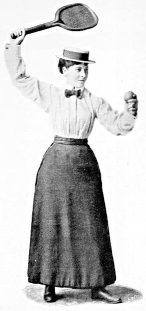
![](https://raw.githubusercontent.com/jacquietran/2019_may_rladies_akl/master/images/illus-310.jpg)
]

.pull-right[
*"For any form of outdoor exercise, the two chief requisites of costume are warmth and lightness. A thin flannel shirt is more useful than anything, worn with a short light skirt."*
]

.footnote[
Image credit: [Project Gutenberg](https://www.gutenberg.org/files/47243/47243-h/47243-h.htm#LAWN-TENNIS)
]

---
background-image: url(https://raw.githubusercontent.com/jacquietran/2019_may_rladies_akl/master/images/sportswomans_lib_frequency.png)
background-size: 85% 80%

---
background-image: url(https://raw.githubusercontent.com/jacquietran/2019_may_rladies_akl/master/images/sportswomans_lib_bigrams.png)
background-size: 85% 80%

---

## R packages used

Project organisation: <a href="https://github.com/jennybc/here_here" target="_blank"><button class="button">here</button></a>

Retrieving text data: <a href="https://github.com/jennybc/here_here" target="_blank"><button class="button">gutenbergr</button></a>

Tidying text data: <a href="https://www.tidytextmining.com/" target="_blank"><button class="button">tidytext</button></a> <a href="https://dplyr.tidyverse.org/" target="_blank"><button class="button">dplyr</button></a> <a href="https://cran.r-project.org/web/packages/stringr/vignettes/stringr.html" target="_blank"><button class="button">stringr</button></a> <a href="https://tidyr.tidyverse.org/" target="_blank"><button class="button">tidyr</button></a>

Creating graph data (for network analysis): <a href="https://igraph.org/r/" target="_blank"><button class="button">igraph</button></a>

Plotting: <a href="https://ggplot2.tidyverse.org/" target="_blank"><button class="button">ggplot2</button></a> <a href="https://github.com/thomasp85/ggraph" target="_blank"><button class="button">ggraph</button></a>

<br />

*****

Code: <a href="https://github.com/jacquietran/2019_may_rladies_akl/blob/master/R/example_text_mining.R" target="_blank"><button class="button_code">On GitHub</button></a>

---
class: inverse, center, middle

# Uses of R in sports analytics

## Example 2: Team scoring dynamics

---
class: center, middle

![](https://raw.githubusercontent.com/jacquietran/2019_may_rladies_akl/master/images/merritt_clauset.PNG)

[**Merritt & Clauset, 2014**](https://link.springer.com/article/10.1140/epjds29), *EPJ Data Science*

---
background-image: url(https://raw.githubusercontent.com/jacquietran/2019_may_rladies_akl/master/images/merritt_clauset_fig3.PNG)
background-size: contain

---
background-image: url(https://raw.githubusercontent.com/jacquietran/2019_may_rladies_akl/master/images/afl_tables_home.PNG)
background-size: cover

---
background-image: url(https://raw.githubusercontent.com/jacquietran/2019_may_rladies_akl/master/images/afl_tables_score_progression.PNG)
background-size: contain

---
class: center, middle

![](https://raw.githubusercontent.com/jacquietran/2019_may_rladies_akl/master/images/tran_letter_header.PNG)

<a href="https://www.jsams.org/article/S1440-2440(17)31300-2/abstract" target="_blank">**Tran & Letter, 2017**</a>, *J Sci Med Sport*

---
class: center, middle
background-image: url(https://raw.githubusercontent.com/jacquietran/2019_may_rladies_akl/master/images/tran_letter_1.png)
background-size: contain

---
class: center, middle
background-image: url(https://raw.githubusercontent.com/jacquietran/2019_may_rladies_akl/master/images/tran_letter_2.png)
background-size: contain

---
class: center, middle
background-image: url(https://raw.githubusercontent.com/jacquietran/2019_may_rladies_akl/master/images/tran_letter_3.png)
background-size: contain

---

## R packages used

Scraping webpage data: <a href="https://blog.rstudio.com/2014/11/24/rvest-easy-web-scraping-with-r/" target="_blank"><button class="button">rvest</button></a>

Tidying data: <a href="https://purrr.tidyverse.org/" target="_blank"><button class="button">purrr</button></a> <a href="https://cran.r-project.org/web/packages/stringr/vignettes/stringr.html" target="_blank"><button class="button">stringr</button></a> <a href="http://had.co.nz/plyr/" target="_blank"><button class="button">plyr</button></a> <a href="https://dplyr.tidyverse.org/" target="_blank"><button class="button">dplyr</button></a> <a href="https://lubridate.tidyverse.org/" target="_blank"><button class="button">lubridate</button></a> <a href="https://seananderson.ca/2013/10/19/reshape/" target="_blank"><button class="button">reshape2</button></a>

Time series analysis: <a href="https://github.com/joshuaulrich/TTR" target="_blank"><button class="button">TTR</button></a> <a href="http://members.cbio.mines-paristech.fr/~thocking/change-tutorial/RK-CptWorkshop.html" target="_blank"><button class="button">changepoint</button></a>

Plotting: <a href="https://ggplot2.tidyverse.org/" target="_blank"><button class="button">ggplot2</button></a>

---
class: inverse, center, middle

# Uses of R in sports analytics

## Example 3: Possession chains

---
class: center, middle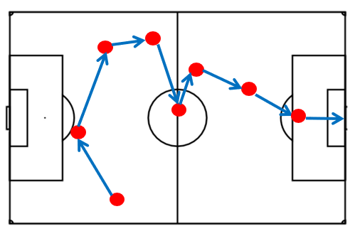

![](https://raw.githubusercontent.com/jacquietran/2019_may_rladies_akl/master/images/di_domenico_soccer.PNG)

---
class: center, middle

---
background-image: url(https://raw.githubusercontent.com/jacquietran/2019_may_rladies_akl/master/images/di_domenico_rationale.png)
background-size: contain

---
background-image: url(https://raw.githubusercontent.com/jacquietran/2019_may_rladies_akl/master/images/di_domenico_header.png)
background-size: contain

---
background-image: url(https://raw.githubusercontent.com/jacquietran/2019_may_rladies_akl/master/images/di_domenico_results_d50.png)
background-size: 80% 90%

---
background-image: url(https://raw.githubusercontent.com/jacquietran/2019_may_rladies_akl/master/images/di_domenico_results_turnovers.png)
background-size: 70% 90%

---

## R packages used

Importing data: <a href="https://readr.tidyverse.org/" target="_blank"><button class="button">readr</button></a>

Tidying data: <a href="http://had.co.nz/plyr/" target="_blank"><button class="button">plyr</button></a>

Decision tree analysis: <a href="https://cran.r-project.org/web/packages/rpart/vignettes/longintro.pdf" target="_blank"><button class="button">rpart</button></a> <a href="https://cran.r-project.org/web/packages/rattle/vignettes/rattle.pdf" target="_blank"><button class="button">rattle</button></a>

Plotting: <a href="https://ggplot2.tidyverse.org/" target="_blank"><button class="button">ggplot2</button></a> <a href="" target="_blank"><button class="button">rpart.plot</button></a> <a href="" target="_blank"><button class="button">RColorBrewer</button></a>

---
class: inverse, center, middle

# Your turn!

---

## Find coding companions! [ 2 min ]

👯 Small groups of **2-3 people**

👋 Connect with **someone you don't know**, or...

🐣 Try for **varied R familiarity** in your group.

👩‍💻 At least **1 laptop per group**, with R and RStudio installed

---

## Set up [ 5 min ]

You'll need these R packages installed and up-to-date for the workshop:

```r
packages <- c(
    'readr',
    'dplyr', 
    'tidyr', 
    'ggplot2',
    'here',
    'usethis'
)

install.packages(packages)
```

---

## Workshop materials

```r
library(usethis)

use_course("https://bit.ly/rladies_sport")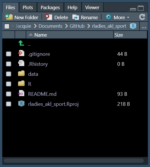
```

![](https://raw.githubusercontent.com/jacquietran/2019_may_rladies_akl/master/images/usethis_1.PNG)

---
class: center, middle

![](https://raw.githubusercontent.com/jacquietran/2019_may_rladies_akl/master/images/usethis_2.PNG)

---
class: center, middle

![](https://raw.githubusercontent.com/jacquietran/2019_may_rladies_akl/master/images/usethis_files.PNG)

---

<br />
This example uses a publicly available data set that includes **all podium results from the Winter Olympic Games from 1924 to 2014, inclusive**.

The `winter` data set is downloadable from this link:  
**[https://www.kaggle.com/the-guardian/olympic-games/data](https://www.kaggle.com/the-guardian/olympic-games/data)**

---

## To help you get started...

In RStudio, use the file explorer to navigate your `rladies_akl_sport` project folder.

---

## To help you get started...

Click on the `R` folder.

Click on the `starter_script.R` file.

---

## Import the data

```r
# The {here} package helps point to a PROJECT-specific file directory,
# rather than a location specific to YOUR personal computer, like:
# C:\Users\YourName\Documents
library(here)

# The {readr} package is efficient for reading (importing) CSVs
library(readr)

# Import the data into your R session
winter <- read_csv(
  here("data/winter.csv"), col_names = TRUE, col_types = NULL)
```

---

## Import the data

```r
# The {here} package helps point to a PROJECT-specific file directory,
# rather than a location specific to YOUR personal computer, like:
# C:\Users\YourName\Documents
*library(here)

# The {readr} package is efficient for reading (importing) CSVs
library(readr)

# Import the data into your R session
winter <- read_csv(
  here("data/winter.csv"), col_names = TRUE, col_types = NULL)
```

---

## Import the data

```r
# The {here} package helps point to a PROJECT-specific file directory,
# rather than a location specific to YOUR personal computer, like:
# C:\Users\YourName\Documents
library(here)

# The {readr} package is efficient for reading (importing) CSVs
*library(readr)

# Import the data into your R session
winter <- read_csv(
  here("data/winter.csv"), col_names = TRUE, col_types = NULL)
```

---

## Import the data

```r
# The {here} package helps point to a PROJECT-specific file directory,
# rather than a location specific to YOUR personal computer, like:
# C:\Users\YourName\Documents
library(here)

# The {readr} package is efficient for reading (importing) CSVs
library(readr)

# Import the data into your R session
*winter <- read_csv(
* here("data/winter.csv"), col_names = TRUE, col_types = NULL)
```

---

## Check the data [ 5 min ]

```r
# Try each of these commands, one-by-one:
head(winter)

str(winter)

dplyr::glimpse(winter)

View(winter)
```

<center>
What do you notice? Which commands do prefer and why?
</center>

---
class: inverse, center, middle

# 'Start with the end in mind.'

---
class: center, middle

## **How many gold medals** were won by
## **Canada, Norway, and Sweden** at the
## **last five Winter Olympic Games**, up to 2014?

---

<br />
To answer this question, we will use R to create this plot:

![](https://raw.githubusercontent.com/jacquietran/2019_essa_forum/master/images/demo1_data_plot.png)

---

## Subset the data

The motivating question: **How many gold medals** were won by **Canada, Norway, and Sweden** at the **last five Winter Olympic Games**, up to 2014?

We need to subset the data to focus only on:

- Gold medal results

- Athletes from Canada (CAN), Norway (NOR), or Sweden (SWE), and

- Results from the five Winter Olympics between 1998 to 2014, inclusive.

---

## Subset the data

```r
# The {dplyr} package includes useful data manipulation functions
*library(dplyr)

# Subset the data
gold_medal_comparison <- winter %>%
  filter(Medal == "Gold"
         & Country %in% c("CAN", "NOR", "SWE")
         & Year >= 1998)
```

---

## Subset the data

```r
# The {dplyr} package includes useful data manipulation functions
library(dplyr)

# Subset the data
*gold_medal_comparison <- winter %>%
  filter(Medal == "Gold"
         & Country %in% c("CAN", "NOR", "SWE")
         & Year >= 1998)
```

---

## Subset the data

```r
# The {dplyr} package includes useful data manipulation functions
library(dplyr)

# Subset the data
gold_medal_comparison <- winter %>%
* filter(Medal == "Gold"
*        & Country %in% c("CAN", "NOR", "SWE")
*        & Year >= 1998)
```

---

## Check the data [ 2 min ]

```r
head(gold_medal_comparison,
*    n = 9)
```

<center>How would you describe the information contained in <b>any one row</b>?</center>

---

## Check the data [ 2 min ]

```r
head(gold_medal_comparison,
*    n = 9)
```

```
## # A tibble: 9 x 9
##    Year City   Sport   Discipline Athlete        Country Gender Event Medal
##   <dbl> <chr>  <chr>   <chr>      <chr>          <chr>   <chr>  <chr> <chr>
## 1  1998 Nagano Biathl~ Biathlon   BJOERNDALEN, ~ NOR     Men    10KM  Gold 
## 2  1998 Nagano Biathl~ Biathlon   HANEVOLD, Hal~ NOR     Men    20KM  Gold 
## 3  1998 Nagano Bobsle~ Bobsleigh  LUEDERS, Pier~ CAN     Men    Two-~ Gold 
## 4  1998 Nagano Bobsle~ Bobsleigh  MACEACHERN, D~ CAN     Men    Two-~ Gold 
## 5  1998 Nagano Curling Curling    BETKER, Jan    CAN     Women  Curl~ Gold 
## 6  1998 Nagano Curling Curling    FORD, Atina    CAN     Women  Curl~ Gold 
## 7  1998 Nagano Curling Curling    GUDEREIT, Mar~ CAN     Women  Curl~ Gold 
## 8  1998 Nagano Curling Curling    MCCUSKER, Joan CAN     Women  Curl~ Gold 
## 9  1998 Nagano Curling Curling    SCHMIRLER, Sa~ CAN     Women  Curl~ Gold
```

---

## Wrangle the data

In the `winter` data set, the data is structured such that **one row is one medal-winning athlete**.

However...

- Team events (e.g., bobsleigh, curling) comprise multiple athletes, and

- Within teams that achieve a podium finish, each athlete is awarded a medal.

For this analysis, we need to wrangle the data to get it into a format where **one row represents one gold medal per event** (rather than per athlete).

---

## Create a new 'identifier' variable

```r
*gold_medal_comparison <- gold_medal_comparison %>%
  mutate(
    unique_event_ID =
      paste(Year, Sport, Discipline, Country, Gender, Event, sep = "_")
    )
```

---

## Create a new 'identifier' variable

```r
gold_medal_comparison <- gold_medal_comparison %>%
* mutate(
    unique_event_ID =
      paste(Year, Sport, Discipline, Country, Gender, Event, sep = "_")
    )
```

---

## Create a new 'identifier' variable

```r
gold_medal_comparison <- gold_medal_comparison %>%
  mutate(
*   unique_event_ID =
      paste(Year, Sport, Discipline, Country, Gender, Event, sep = "_")
    )
```

---

## Create a new 'identifier' variable

```r
gold_medal_comparison <- gold_medal_comparison %>%
  mutate(
    unique_event_ID =
*     paste(Year, Sport, Discipline, Country, Gender, Event, sep = "_")
    )
```

---

## Create a new 'identifier' variable

```r
gold_medal_comparison <- gold_medal_comparison %>%
  mutate(
    unique_event_ID =
      paste(Year, Sport, Discipline, Country, Gender, Event, sep = "_")
*   )
```

---

## Check the new variable

```r
gold_medal_comparison %>%
* select(unique_event_ID)
```

What do you notice?

---

## Check the new variable

```r
gold_medal_comparison %>%
* select(unique_event_ID)
```

```
## # A tibble: 358 x 1
##    unique_event_ID                                           
##    <chr>                                                     
##  1 1998_Biathlon_Biathlon_NOR_Men_10KM                       
##  2 1998_Biathlon_Biathlon_NOR_Men_20KM                       
##  3 1998_Bobsleigh_Bobsleigh_CAN_Men_Two-Man                  
##  4 1998_Bobsleigh_Bobsleigh_CAN_Men_Two-Man                  
##  5 1998_Curling_Curling_CAN_Women_Curling                    
##  6 1998_Curling_Curling_CAN_Women_Curling                    
##  7 1998_Curling_Curling_CAN_Women_Curling                    
##  8 1998_Curling_Curling_CAN_Women_Curling                    
##  9 1998_Curling_Curling_CAN_Women_Curling                    
## 10 1998_Skating_Short Track Speed Skating_CAN_Men_5000M Relay
## # ... with 348 more rows
```

---

## Check the new variable

```r
gold_medal_comparison %>%
  select(unique_event_ID)
```

```
## # A tibble: 358 x 1
##    unique_event_ID                                           
##    <chr>                                                     
##  1 1998_Biathlon_Biathlon_NOR_Men_10KM                       
##  2 1998_Biathlon_Biathlon_NOR_Men_20KM                       
*##  3 1998_Bobsleigh_Bobsleigh_CAN_Men_Two-Man                  
*##  4 1998_Bobsleigh_Bobsleigh_CAN_Men_Two-Man                  
##  5 1998_Curling_Curling_CAN_Women_Curling                    
##  6 1998_Curling_Curling_CAN_Women_Curling                    
##  7 1998_Curling_Curling_CAN_Women_Curling                    
##  8 1998_Curling_Curling_CAN_Women_Curling                    
##  9 1998_Curling_Curling_CAN_Women_Curling                    
## 10 1998_Skating_Short Track Speed Skating_CAN_Men_5000M Relay
## # ... with 348 more rows
```

---

## Check the new variable

```r
gold_medal_comparison %>%
  select(unique_event_ID)
```

```
## # A tibble: 358 x 1
##    unique_event_ID                                           
##    <chr>                                                     
##  1 1998_Biathlon_Biathlon_NOR_Men_10KM                       
##  2 1998_Biathlon_Biathlon_NOR_Men_20KM                       
##  3 1998_Bobsleigh_Bobsleigh_CAN_Men_Two-Man                  
##  4 1998_Bobsleigh_Bobsleigh_CAN_Men_Two-Man                  
*##  5 1998_Curling_Curling_CAN_Women_Curling                    
*##  6 1998_Curling_Curling_CAN_Women_Curling                    
*##  7 1998_Curling_Curling_CAN_Women_Curling                    
*##  8 1998_Curling_Curling_CAN_Women_Curling                    
*##  9 1998_Curling_Curling_CAN_Women_Curling                    
## 10 1998_Skating_Short Track Speed Skating_CAN_Men_5000M Relay
## # ... with 348 more rows
```

---

## Identify duplicate event IDs

```r
gold_medal_comparison %>%
* mutate(duplicates = duplicated(unique_event_ID)) %>%
  select(unique_event_ID, duplicates) %>%
  head(n = 7)
```

```
## # A tibble: 7 x 2
##   unique_event_ID                          duplicates
##   <chr>                                    <lgl>     
## 1 1998_Biathlon_Biathlon_NOR_Men_10KM      FALSE     
## 2 1998_Biathlon_Biathlon_NOR_Men_20KM      FALSE     
## 3 1998_Bobsleigh_Bobsleigh_CAN_Men_Two-Man FALSE     
## 4 1998_Bobsleigh_Bobsleigh_CAN_Men_Two-Man TRUE      
## 5 1998_Curling_Curling_CAN_Women_Curling   FALSE     
## 6 1998_Curling_Curling_CAN_Women_Curling   TRUE      
## 7 1998_Curling_Curling_CAN_Women_Curling   TRUE
```

---

## Identify duplicate event IDs

```r
gold_medal_comparison %>%
  mutate(duplicates = duplicated(unique_event_ID)) %>%
  select(unique_event_ID, duplicates) %>%
  head(n = 7)
```

```
## # A tibble: 7 x 2
##   unique_event_ID                          duplicates
##   <chr>                                    <lgl>     
## 1 1998_Biathlon_Biathlon_NOR_Men_10KM      FALSE     
## 2 1998_Biathlon_Biathlon_NOR_Men_20KM      FALSE     
## 3 1998_Bobsleigh_Bobsleigh_CAN_Men_Two-Man FALSE     
*## 4 1998_Bobsleigh_Bobsleigh_CAN_Men_Two-Man TRUE      
## 5 1998_Curling_Curling_CAN_Women_Curling   FALSE     
*## 6 1998_Curling_Curling_CAN_Women_Curling   TRUE      
*## 7 1998_Curling_Curling_CAN_Women_Curling   TRUE
```

---

## Omit rows with duplicate IDs

```r
*gold_medal_comparison <- gold_medal_comparison %>%
  mutate(duplicates = duplicated(unique_event_ID)) %>%
  filter(duplicates == FALSE) %>%
  select(Year, City, Sport, Country, Event, Medal)
```

---

## Omit rows with duplicate IDs

```r
gold_medal_comparison <- gold_medal_comparison %>%
* mutate(duplicates = duplicated(unique_event_ID)) %>%
  filter(duplicates == FALSE) %>%
  select(Year, City, Sport, Country, Event, Medal)
```

---

## Omit rows with duplicate IDs

```r
gold_medal_comparison <- gold_medal_comparison %>%
  mutate(duplicates = duplicated(unique_event_ID)) %>%
* filter(duplicates == FALSE) %>%
  select(Year, City, Sport, Country, Event, Medal)
```

---

## Omit rows with duplicate IDs

```r
gold_medal_comparison <- gold_medal_comparison %>%
  mutate(duplicates = duplicated(unique_event_ID)) %>%
  filter(duplicates == FALSE) %>%
* select(Year, City, Sport, Country, Event, Medal)
```

```
## # A tibble: 6 x 6
##    Year City   Sport     Country Event       Medal
##   <dbl> <chr>  <chr>     <chr>   <chr>       <chr>
## 1  1998 Nagano Biathlon  NOR     10KM        Gold 
## 2  1998 Nagano Biathlon  NOR     20KM        Gold 
## 3  1998 Nagano Bobsleigh CAN     Two-Man     Gold 
## 4  1998 Nagano Curling   CAN     Curling     Gold 
## 5  1998 Nagano Skating   CAN     5000M Relay Gold 
## 6  1998 Nagano Skating   CAN     500M        Gold
```

---

## Omit rows with duplicate IDs

```r
gold_medal_comparison <- gold_medal_comparison %>%
  mutate(duplicates = duplicated(unique_event_ID)) %>%
  filter(duplicates == FALSE) %>%
  select(Year, City, Sport, Country, Event, Medal)
```

```
## # A tibble: 6 x 6
##    Year City   Sport     Country Event       Medal
##   <dbl> <chr>  <chr>     <chr>   <chr>       <chr>
## 1  1998 Nagano Biathlon  NOR     10KM        Gold 
## 2  1998 Nagano Biathlon  NOR     20KM        Gold 
*## 3  1998 Nagano Bobsleigh CAN     Two-Man     Gold 
## 4  1998 Nagano Curling   CAN     Curling     Gold 
## 5  1998 Nagano Skating   CAN     5000M Relay Gold 
## 6  1998 Nagano Skating   CAN     500M        Gold
```

---

## Omit rows with duplicate IDs

```r
gold_medal_comparison <- gold_medal_comparison %>%
  mutate(duplicates = duplicated(unique_event_ID)) %>%
  filter(duplicates == FALSE) %>%
  select(Year, City, Sport, Country, Event, Medal)
```

```
## # A tibble: 6 x 6
##    Year City   Sport     Country Event       Medal
##   <dbl> <chr>  <chr>     <chr>   <chr>       <chr>
## 1  1998 Nagano Biathlon  NOR     10KM        Gold 
## 2  1998 Nagano Biathlon  NOR     20KM        Gold 
## 3  1998 Nagano Bobsleigh CAN     Two-Man     Gold 
*## 4  1998 Nagano Curling   CAN     Curling     Gold 
## 5  1998 Nagano Skating   CAN     5000M Relay Gold 
## 6  1998 Nagano Skating   CAN     500M        Gold
```

---

## Calculate gold medal totals

Now that we have tidied up the data into the format we need, we can calculate the **total number of gold medals** won by **Canada, Norway, and Sweden** at each of the **Winter Games between 1998 and 2014**.

---

## Calculate gold medal totals

```r
# Calculate total number of gold medals per team per Winter Games
*gold_medal_totals <- gold_medal_comparison %>%
  group_by(Year, City, Country) %>%
  summarise(gold_medal_total = length(Medal)) %>%
  ungroup()
```

---

## Calculate gold medal totals

```r
# Calculate total number of gold medals per team per Winter Games
gold_medal_totals <- gold_medal_comparison %>%
* group_by(Year, City, Country) %>%
  summarise(gold_medal_total = length(Medal)) %>%
  ungroup()
```

---

## Calculate gold medal totals

```r
# Calculate total number of gold medals per team per Winter Games
gold_medal_totals <- gold_medal_comparison %>%
  group_by(Year, City, Country) %>%
* summarise(gold_medal_total = length(Medal)) %>%
  ungroup()
```

---

## Calculate gold medal totals

```r
# Calculate total number of gold medals per team per Winter Games
gold_medal_totals <- gold_medal_comparison %>%
  group_by(Year, City, Country) %>%
  summarise(gold_medal_total = length(Medal)) %>%
* ungroup()
```

---

## Calculate gold medal totals

When we check the data, we can see it is in long format:

```r
gold_medal_totals
```

```
## # A tibble: 13 x 4
##     Year City           Country gold_medal_total
##    <dbl> <chr>          <chr>              <int>
##  1  1998 Nagano         CAN                    6
##  2  1998 Nagano         NOR                   10
##  3  2002 Salt Lake City CAN                    8
##  4  2002 Salt Lake City NOR                   12
##  5  2006 Turin          CAN                    7
##  6  2006 Turin          NOR                    2
##  7  2006 Turin          SWE                    7
##  8  2010 Vancouver      CAN                   15
##  9  2010 Vancouver      NOR                    9
## 10  2010 Vancouver      SWE                    5
## 11  2014 Sochi          CAN                   10
## 12  2014 Sochi          NOR                   12
## 13  2014 Sochi          SWE                    2
```

---

We can use the gold medal totals to produce **this plot**, using a popular R package called `ggplot2`:

![](https://raw.githubusercontent.com/jacquietran/2019_essa_forum/master/images/demo1_data_plot.png)

---

## gg = Grammar of Graphics

`ggplot2` draws upon a **layered Grammar of Graphics** as a theoretical foundation for how to make plots (Wilkinson et al., 2005; Wickham, 2010).

.footnote[
[1] Wilkinson et al., 2005, _['The Grammar of Graphics'](https://www.amazon.com/Grammar-Graphics-Statistics-Computing/dp/0387245448)_.

[2] Wickham, 2010, ['A layered grammar of graphics'](https://vita.had.co.nz/papers/layered-grammar.html), _Journal of Computational and Graphical Statistics_
]

---
class: center, middle

![](https://raw.githubusercontent.com/jacquietran/2019_essa_forum/master/images/gg_fig1.PNG)

Wickham, 2010, **['A layered grammar of graphics'](https://vita.had.co.nz/papers/layered-grammar.html)**

---
class: center, middle

Wickham, 2010, **['A layered grammar of graphics'](https://vita.had.co.nz/papers/layered-grammar.html)**

---

## Start afresh!

From RStudio's top navigation bar,

- Go to the **Session** menu
- Click **Clear Workspace**
- Open the **Session** menu again
- Click **Restart R**.

---

## Another helper script!

In RStudio, use your file explorer to find and open the `plot_helper.R` script.

---

## Load packages

```r
# Load libraries
# The {ggplot2} package is a powerful, feature-rich
# R package for creating data visualisations
library(ggplot2)
library(here)
```

---

## Import the wrangled data

```r
# Use this code to import the wrangled data set
# that's ready for you to plot!
gold_medal_totals <- readRDS(here("data/gold_medal_totals.rds"))
```

---

## Plot the data

```r
# Start building the plot, layer-by-layer
p <- ggplot(data = gold_medal_totals,
            aes(x = Year, y = gold_medal_total,
                fill = Country))
p <- p + geom_bar(stat = "identity")
```

---

## Plot the data

```r
# Start building the plot, layer-by-layer
*p <- ggplot(data = gold_medal_totals,
            aes(x = Year, y = gold_medal_total,
                fill = Country))
p <- p + geom_bar(stat = "identity")
```

---

## Plot the data

```r
# Start building the plot, layer-by-layer
p <- ggplot(data = gold_medal_totals,
*           aes(x = Year, y = gold_medal_total,
                fill = Country))
p <- p + geom_bar(stat = "identity")
```

---

## Plot the data

```r
# Start building the plot, layer-by-layer
p <- ggplot(data = gold_medal_totals,
            aes(x = Year, y = gold_medal_total,
*               fill = Country))
p <- p + geom_bar(stat = "identity")
```

---

## Plot the data

```r
# Start building the plot, layer-by-layer
p <- ggplot(data = gold_medal_totals,
            aes(x = Year, y = gold_medal_total,
                fill = Country))
*p <- p + geom_bar(stat = "identity")
```

To display the plot, call the object `p`:

```r
p
```

---
class: center, middle

![](presentation_files/figure-html/demo1_display_plot_1b-1.png)

It's a start, but...how could we improve this plot?

---

## Areas for improvement

Show countries side-by-side (rather than stacked)

Informative plot and axis titles

Clearer axis breaks

Colourblind-friendly palette

Larger font sizes

---

## Countries shown side-by-side

To the previous code chunk we started as the base for this plot, we **add layers** to specify modifications to the plot:

```r
p <- p + facet_wrap(~Country, nrow = 1)
```

Then we **select the whole ggplot code chunk** (i.e., all layers) and run the code to re-build the plot.

---
class: center, middle

![](presentation_files/figure-html/demo1_display_plot_2-1.png)

A bit better, but now the legend is redundant, so we can add it to our 'to do' list.

---

## Areas for improvement

~~Show countries side-by-side (rather than stacked)~~

Informative plot and axis titles

Clearer x axis breaks

Colourblind-friendly palette

Larger font sizes

Remove legend

---

## Informative titles

```r
p <- p + labs(
  title = "Canada increased its Winter Games gold medal haul over 20 years",
  x = "Year",
  y = "Total # of gold medals won")
```

---

![](presentation_files/figure-html/demo1_display_plot_3-1.png)

---

## Areas for improvement

~~Show countries side-by-side (rather than stacked)~~

~~Informative plot and axis titles~~

Clearer x axis breaks

Colourblind-friendly palette

Larger font sizes

Remove legend

---

## Clearer x axis breaks

```r
p <- p + scale_x_continuous(
  limits = c(1996,2016),
  breaks = seq(1998,2014, by = 4))
```

---

![](presentation_files/figure-html/demo1_display_plot_4-1.png)

---

## Areas for improvement

~~Show countries side-by-side (rather than stacked)~~

~~Informative plot and axis titles~~

~~Clearer x axis breaks~~

Colourblind-friendly palette

Larger font sizes

Remove legend

---

## Colourblind-friendly palette

_'As many as 8% of men and 0.5 of women with Northern European ancestry have the common form of red-green color blindness.'_ - National Eye Institute, 2015

```r
# The {dichromat} package contains 17 palettes that are
# "suitable for people with deficient or anomalous red-green vision"
library(dichromat)
```

.footnote[
[1] National Eye Institute, 2015, ['Facts about color blindness'](https://nei.nih.gov/health/color_blindness/facts_about).

[2] University of British Columbia, ['Using colors in R: Accommodating color blindness'](http://stat545.com/block018_colors.html#accomodating-color-blindness), _STAT 545 course materials_.
]

---
class: center, middle

![](https://raw.githubusercontent.com/jacquietran/2019_essa_forum/master/images/dichromat-colorschemes-1.png)

STAT 545: **[Using colors in R](http://stat545.com/block018_colors.html#accomodating-color-blindness)**

---

## Colourblind-friendly palette

```r
p <- p + scale_fill_manual(
  values = c(
    "CAN" = colorschemes$BluetoGray.8[1],
    "NOR" = colorschemes$BluetoGray.8[2],
    "SWE" = colorschemes$BluetoGray.8[7]))
```

---

![](presentation_files/figure-html/demo1_display_plot_5-1.png)

---

## Areas for improvement

~~Show countries side-by-side (rather than stacked)~~

~~Informative plot and axis titles~~

~~Clearer x axis breaks~~

~~Colourblind-friendly palette~~

Larger font sizes

Remove legend

---

## Larger font sizes

```r
# Change the base font size for all text elements
p <- p + theme(
  text = element_text(size = 28))
```

---

![](presentation_files/figure-html/demo1_display_plot_6-1.png)

Notice that the different text elements show a hierarchy of font sizes.

---

# Areas for improvement

~~Show countries side-by-side (rather than stacked)~~

~~Informative plot and axis titles~~

~~Clearer x axis breaks~~

~~Colourblind-friendly palette~~

~~Larger font sizes~~

Remove legend

---

## Remove legend

```r
# Change the base font size for all text elements
p <- p + theme(
  text = element_text(size = 28),
* legend.position = "none")
```

---
class: center, middle

![](presentation_files/figure-html/demo1_display_plot_7-1.png)

We're done with our major improvements!

---

## Change position of titles

With our last few tweaks, we can improve readability by increasing the whitespace between the titles and the plot area.

```r
p <- p + theme(
  text = element_text(size = 28),
  legend.position = "none",
* plot.title = element_text(margin = margin(b = 15, unit = "pt")),
* axis.title.x = element_text(margin = margin(t = 15, unit = "pt")),
* axis.title.y = element_text(margin = margin(r = 15, unit = "pt")))
```

---
class: center, middle

![](presentation_files/figure-html/demo1_display_plot_8-1.png)

All done!

---
class: inverse, center, middle

# Develop your data proficiency
## Resources to get you started

---

- [**Data organisation in spreadsheets**](https://www.tandfonline.com/doi/abs/10.1080/00031305.2017.1375989)

Karl Broman & Kara Woo, 2018, *The American Statistician*, *72*(1).

- [**Installing R and RStudio**](https://rstudio-education.github.io/hopr/starting.html)

From the [**Hands on Programming with R**](https://rstudio-education.github.io/hopr/) book by Garrett Grolemund (@StatGarrett).
  
--

- [**STAT 545: Data wrangling, exploration, and analysis with R**](https://stat545.com/)
  
  Open course materials produced by faculty at the University of British Columbia

- [**Chromebook Data Science**](https://jhudatascience.org/chromebookdatascience/)
  
  Open course materials produced by faculty at Johns Hopkins University
  
--

- [**R for Data Science**](https://r4ds.had.co.nz/)
  
  Book written by Garrett Grolemund (@StatGarrett) & Hadley Wickham (@hadleywickham). Free online, hard copy available for purchase.

---
class: inverse, center, middle